The usability of Bayesian networks
Statistics! No matter what you think about it, no matter if you like it or not, you cannot say that statistics isn’t useful! If you haven’t worked with stati...
Originally posted on 2014-04-18. Since this was first written, GeNIe has been acquired by BayesFusion and is unfortunately no longer freeware.
Statistics! No matter what you think about it, no matter if you like it or not, you cannot say that statistics isn’t useful! If you haven’t worked with statistics very much, some of it may feel a little blurry but when it comes to modeling uncertainty, you can’t get away from probabilities. This post will be about a particular branch of statistics called Bayesian probability. To be more precise, it will be about the statistical model called Bayesian networks. But first we need a bit of background. If you feel like you know what bayesian probability is all about, you should be able to skip this.
Thomas Bayes was a British statistician, most famous for formulating the theorem called Bayes' theorem. In its simplest form, the theorem looks like this:

P(A|B) should be read as “the probability of A being true, under the condition that B is true”.
What the theorem says is basically that under the condition that B is true, the probability of A also being true is equal to the probability of B being true under the condition that A is true, times the probability of A being true (no matter what B is), divided by the probability of B being true (no matter what A is).
If this sounds like complete mumbo jumbo to you, you aren’t alone. To make it easier to understand the theorem I will present a little example (completely made up!).
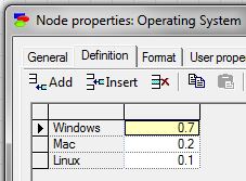
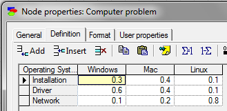
Imagine that you’re running a help desk service. Of the people calling you, 70 % use Windows, 20 % use Mac and 10 % use Linux. You also know that of the Windows users, 30 % have problems installing a program, 60 % have driver problems and 10 % have network configuration problems. Of the Mac users, 40 % have program installation problems, 40 % have driver problems and 20 % have problems configuring their network settings. Lastly, of the Linux users, 10 % have problems installing a program, 10 % have driver problems and 80 % have network configuration problems.
Now, say that Peter needs help and calls you. Before he explains his problem to you, the likelihood that he uses Linux is pretty small, only ten percent (as described above). But if Peter tells you that he experiences problems with his network configuration, is the probability of him using Linux still 10 %? It turns out that if you include this new information into your analysis, the probability of Peter being a Linux user rises to 42 %!
The reason for this is that the first question we asked was “what is the probability that Peter uses Linux?” while the other question was “what is the probability that Peter uses Linux if we know that he has network configuration problems?”. To make the following equations more readable, let us say that:
From the text we also know that
P(W) = 0.7, P(M) = 0.2, P(L) = 0.1 (probabilities for using the different OSes)P(K|W) = 0.3, P(D|W) = 0.6, P(N|W) = 0.1 (different problems under Windows)P(K|M) = 0.4, P(D|M) = 0.4, P(N|M) = 0.2 (different problems under Mac)P(K|L) = 0.1, P(D|L) = 0.1, P(N|L) = 0.8 (different problems under Linux)The question “what is the probability that Peter uses Linux?” then means calculating P(L) = 0.1, while “what is the probability that Peter uses Linux if we know that he has network configuration problems?” means calculating P(L|N). Even though we haven’t said anything about what P(L|N) might be, we can calculate it using Bayes’ theorem!

By changing A and B to our own variables {W, M, L, K, D, N} we get

We already know what P(N|L) is, and we already know P(L), but the text doesn’t say anything about P(N). We can, however, calculate it. Since P(N) is “the probability that a user has network problems” it is the same as the summed probabilities P(N) = P(N|W)*P(W) + P(N|M)*P(M) + P(N|L)*P(L). The likelihood that Peter is a Linux user thus becomes

And when the likelihood of Peter using Linux increased from 10 % to 42 %, the likelihood of him being a Windows user decreased from 70 % to about 37 % while Mac stayed almost the same, a small increase from 20 % to 21 %. By using Bayesian inference it is possible to make use of extra information to make more accurate guesses about one’s environment. This method is for example used by so called Expert systems to make medical diagnoses.
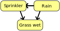
The probabilistic model called Bayesian networks (or belief networks) makes, as the name suggests, heavy use of Bayesian probability. A bayesian network can be thought of as a visualisation of probabilities that in some way or another depend on eachother. A simple example (nicely presented on the Wikipedia article on Bayesian networks) is the relationship between rain, sprinkler usage and wet grass. The usage of a sprinkler depends on whether it has rained or not (which is why there is an arrow from the node ‘Rain’ to ‘Sprinkler’), and the presence of wet grass depends both on whether a sprinkler has been used and whether it has rained or not (the arrows that go to ‘Grass wet’).
There are many programs developed for using Bayesian networks, one of which is GeNIe (Graphical Network Interface) developed by the Decision Systems Laboratory at the University of Pittsburgh. GeNIe has a pretty intuitive graphical interface and uses the C++ library called SMILE (also developed by the Decision Systems Laboratory) as a backend. Additionally, SMILE can be used as an independent library for Bayesian networks, something that allows developers to create programs that make use of Bayesian networks.
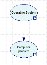
The previous example of computer problems which depend on the user’s operating system can be visualised by using GeNIe. As can be seen in the picture below, only two nodes are required. The ‘Operating System’ node contains three states; ‘Windows’, ‘Mac’ and ‘Linux’. The ‘Computer problem’ node also contains three states; ‘Installation’, ‘Driver’ and ‘Network’.
The known probabilities for each node are entered in the node properties.
When the Bayesian network has been set up, it’s possible to set the observed evidence (the user had a network problem) and update the network. By then holding the mouse over the nodes, GeNIe displays the calculated probabilities (which gives the same results as our own “manual” calculations!).
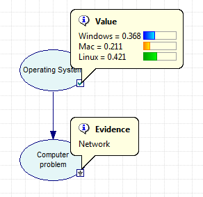
This method is a bit easier than, as we did above, doing all the calculations by hand. And by using SMILE (or any other library for Bayesian networks) in the programs you create, you too can exploit the usability of Bayesian networks!
Statistics! No matter what you think about it, no matter if you like it or not, you cannot say that statistics isn’t useful! If you haven’t worked with stati...
Imagine that you’re standing in your living room with your eyes closed. Now, you might have a mental map of the room and where the furniture are, but would y...
Yay! At last! The old ‘work-in-progress’ HTML site is gone from plankter.se, and instead this is here. Everything is not in place yet. I am still missing the...
Right, so I’m working on updating my website to a working condition again and am testing a framework called Jekyll.